Classification Tree

Supervised Learning Model

Tree models where the target variable can take a finite set of
values are called classification trees.
Decision trees where the target variable can take continuous values (typically real numbers) are called regression trees.

In this example, target is categorical variable and features used to predict are numerical variables.

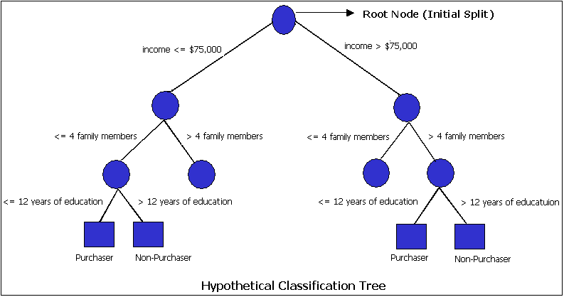
ctree1
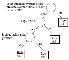
ctree2
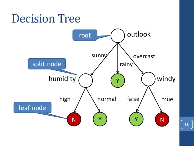
distributed-decision-tree-learning-for-mining-big-data-streams-16-638

Programming Logic

Steps to build classification tree model to predict a categorical target variable based on numerical feature variables

Pre-requisite:

Understand the data set for pre-processing that may be requierd to create sample dataset for training and testing.

Step 1:
Install the required R packages and load them

Step 2:
Set up the environment options, if any
Set seed

Step 3:
Create train and test data from data set
Use 70% for training the model and remaing for testing

Step 4:
Define the formula for predicting target variable based on feature variables
Build classification tree model using the formula and the train data set

Step 5:
Cross check the model by predicting training data target variable
Predictions should match accurately since the model is built using the same training data

Step 6:
Print the classification tree model for better understanding

Step 7:
Plot the classification tree model and interpret the tree structure

Step 8:
Now use the classification tree model to predict the target for test data.

Step 9:
Determine the accuracy of the model for the predictions of test data target variable.

Understanding data set

We use the inbuilt data set iris.

It has 150 observations and 5 variables. We need to build a model to predict the categorical target variable 'Species' using the numerical feature variables Petal.Length, Petal.Width, Sepal.Length, Sepal.Width

# check dimensions of data set

dim(iris)
# [1] 150 5

names(iris)
#[1] "Sepal.Length" "Sepal.Width" "Petal.Length" "Petal.Width" "Species"

str(iris)
#'data.frame': 150 obs. of 5 variables:
# $ Sepal.Length: num 5.1 4.9 4.7 4.6 5 5.4 4.6 5 4.4 4.9 ...
# $ Sepal.Width : num 3.5 3 3.2 3.1 3.6 3.9 3.4 3.4 2.9 3.1 ...
# $ Petal.Length: num 1.4 1.4 1.3 1.5 1.4 1.7 1.4 1.5 1.4 1.5 ...
# $ Petal.Width : num 0.2 0.2 0.2 0.2 0.2 0.4 0.3 0.2 0.2 0.1 ...
# $ Species : Factor w/ 3 levels "setosa","versicolor",..: 1 1 1 1 1 1 1 1 1 1 ...

Install required R packages 


install.packages("party")

Load installed R packages

libs = c("party")
lapply(libs, require, character.only=TRUE)


Set seed

To make result reproducible

set.seed(1234)

Create train and test data set

Split the data set in to two parts - 70% for training and remaining 30% for testing


Use sample function to shuffle the dataset and assign index 1 to 70% of data and index 2 to remaining data points; such that index 1 can be used as training set and 2 as testing set


#sample the data by assigning index positions

ind = sample(2, nrow(iris), replace=TRUE, prob=c(0.7,0.3))
str(ind)
# int [1:150] 2 1 1 1 1 1 2 1 2 1 ...

# train dataset is all rows with index 1, 70% of dataset

trainData = iris[ind==1,]
str(trainData)
# 'data.frame': 96 obs. of 5 variables:
# $ Sepal.Length: num 4.9 4.7 4.6 5 5.4 5 4.9 5.4 4.8 5.8 ...
# $ Sepal.Width : num 3 3.2 3.1 3.6 3.9 3.4 3.1 3.7 3.4 4 ...
# $ Petal.Length: num 1.4 1.3 1.5 1.4 1.7 1.5 1.5 1.5 1.6 1.2 ...
# $ Petal.Width : num 0.2 0.2 0.2 0.2 0.4 0.2 0.1 0.2 0.2 0.2 ...
# $ Species : Factor w/ 3 levels "setosa","versicolor",..: 1 1 1 1 1 1 1 1 1 1 ...

# test dataset is all rows with index 2, 30% of dataset

testData = iris[ind==2,]
str(testData)
# 'data.frame': 54 obs. of 5 variables:
# $ Sepal.Length: num 5.1 4.6 4.4 4.8 4.3 5.1 5.1 4.6 4.8 5 ...
# $ Sepal.Width : num 3.5 3.4 2.9 3 3 3.8 3.7 3.6 3.4 3 ...
# $ Petal.Length: num 1.4 1.4 1.4 1.4 1.1 1.5 1.5 1 1.9 1.6 ...
# $ Petal.Width : num 0.2 0.3 0.2 0.1 0.1 0.3 0.4 0.2 0.2 0.2 ...
# $ Species : Factor w/ 3 levels "setosa","versicolor",..: 1 1 1 1 1 1 1 1 1 1 #...

Define formula to predict target variable

Use this formula to build the classification tree model for prediction:

Species ~ Sepal.Length + Sepal.Width + Petal.Length + Petal.Width

# target depends on all features use dot '.' to indicate all features as predictors

myFormula = Species ~ .
str(myFormula)
# Class 'formula' length 3 Species ~ Sepal.Length + Sepal.Width + Petal.Length + Petal.Width
# ..- attr(*, ".Environment")=<environment: R_GlobalEnv>

# use ctree function to build classification tree model

iris_ctree = ctree(myFormula, data=trainData)
str(iris_ctree)
# Formal class 'BinaryTree' [package "party"] with 10 slots
# ..@ data :Formal class 'ModelEnvFormula' [packa
# and so on

Cross check the prediction model

Since the model is built using training data, it should predict target values for training set accurately


# checking prediction model with the train data

trainPred = predict(iris_ctree, data=trainData)

# confusion matrix for predicted and actual values

table(trainPred, trainData$Species)
#trainPred   setosa   versicolor   virginica
#setosa            35          0                  0
#versicolor      0            28                0
#virginica        0            4                   29

Understanding the classification tree model

*weights - are the predictions

Add up the nodes 2, 4, 5 ( 35 + 28 + 33) equals the total observations 96

1, 3 are the split conditions resulting in either a prediction node or another split condition

Plot the tree to see the split condition

# print the decision model

print(iris_ctree)

# Conditional inference tree with 3 terminal nodes

.

# Response: Species
# Inputs: Sepal.Length, Sepal.Width, Petal.Length, Petal.Width
# Number of observations: 96

.

# 1) Petal.Length <= 1.9; criterion = 1, statistic = 91.329
# 2)* weights = 35
# 1) Petal.Length > 1.9
# 3) Petal.Length <= 4.7; criterion = 1, statistic = 39.298
# 4)* weights = 28
# 3) Petal.Length > 4.7
# 5)* weights = 33

Plot the classification tree

plot(iris_ctree)

Interpret the classification tree plot

It is an upside-down tree following the pattern:
Root condition for binary split, each branch ending in to a node/prediction or growing the tree with another split condition
In this plot, root condition is Petal.Length, binary split <= 1.9 ending in node or prediction sentosa for 35 observations the other branch with split condition for Petal.Length <= 4.7 and so on

classification-tree

Use the model to predict test data target

Here we predict the Species for the test data using the classification tree model that was built using the training data

# now use the ctree model to predict Species for test dataset

testPred = predict(iris_ctree, newdata=testData)
testPred
# [1] setosa setosa setosa setosa setosa
# [6] setosa setosa setosa setosa setosa
# [11] setosa setosa setosa setosa setosa
# [16] versicolor versicolor versicolor versicolor versicolor
# [21] versicolor virginica versicolor versicolor virginica
# [26] versicolor versicolor versicolor versicolor versicolor
# [31] versicolor versicolor versicolor virginica virginica
# [36] versicolor virginica virginica virginica virginica
# [41] virginica virginica virginica virginica virginica
# [46] virginica virginica virginica virginica virginica
# [51] virginica virginica virginica virginica
# Levels: setosa versicolor virginica

str(testPred)
# Factor w/ 3 levels "setosa","versicolor",..: 1 1 1 1 1 1 1 1 1 1 ...

Compare predicted and actual values using confusion matrix

Interpreting the confusion matrix

- vertical values are predicted for target Species
- horizontal values are actuals for target Species
- diagonal cells are correct predictions - matching the actuals

# 15 sentosas correctly predicted as sentosa
# 16 versicolor correctly predicted as versicolor
# 20 virginica correctly predicted as virginica

- non-zero non-diagonal cells are the errors

# 1 virginica wrongly predicted as versicolor
# 2 versicolor wrongly predicted as virginica

#compare the predicted value with the actual value

table(testPred, testData$Species)

# testPred      setosa versicolor virginica
# setosa             15           0              0
# versicolor        0           16             1
# virginica           0            2             20

Determine accuracy of model

Based on the predictions on test data accuracy is calculated as the mean of correct predictions for the target variable Species

#calculate accuracy of prediction

accuracy = mean(testPred == testData$Species)
accuracy
#[1] 0.9444444

error = mean(testPred != testData$Species)
error
#[1] 0.05555556